Encoding Problems in Boolean Satisfiability
The Boolean Satisfiability Problem (SAT, for short) is one of the most famous problems in computer science. Given a logical statement in propositional logic, it asks for an assignment to the Boolean variables that “satisfies” the statement. In this post, we will explore how we can use SAT as a programming paradigm to solve combinatorial problems. In the rest of this post, I will assume that the reader has basic understanding of propositional logic (i.e., mostly what a “proposition” means, and also what “or”, “and”, “implies”, and similar operators mean).
As an example, given a logical statement “\(p\) or \(q\)”, a satisfying assignment is “\(p =\) True”. In this case, we say that this formula is “satisfiable”. As another example, the formula “\(p\) and not \(p\)” is not satisfiable, since regardless of what we assign to \(p\), the statement’s truth value will be False.
It turns out that due to Cook’s Theorem, all problems in NP can be represented as such a formula, and we can use a SAT solver to find the solution to the problem. This makes SAT not only a theoretical problem in computer science, but also a powerful programming paradigm for solving hard decision problems.
Somewhat formal definitions
Before we dive into how we can solve a practical problem with this paradigm, there are some definitions and notations we will have to fix.
- In propositional logic, we have two constant values, which are “top” (\(\top\)), and “bottom” (\(\bot\)). \(\top\) always evaluates to True, and \(\bot\) always evaluates to False.
- A variable is something that we can assign to either True or False. We usually use the letters \(p,q,r\) to denote variables.
- A variable can be negated with the unary operator \(\neg\). For instance, the negation of the variable \(p\) is \(\neg p\).
- A variable, or the negation of a variable is called a “literal”. For instance, \(p, q, \neg q, \neg r\) are all literals.
It is worth pointing out that variables and literals do not mean anything by themselves, it is us who associate real world meanings with them. For instance, in my world \(p\) can mean that today is sunny, and the meaning I associate with it does not change whether a certain formula over \(p\) is satisfiable or not.
Next, we have some recursive definitions concerning “propositional formulas”. These are complex propositions that we can express with literals using a few operators. We reserve the letters \(F,G,H,\ldots\) to denote formulas. In the following we describe the precise set of formulas:
- \(\top\) and \(\bot\) are formulas
- A literal is a formula
- “And” of two formulas \(F\) and \(G\) is a formula, denoted as (\(F \wedge G\)). Such a formula is also called a “conjunction”.
- “Or” of two formulas \(F\) and \(G\) is a formula, denoted as \((F \vee G)\). Such a formula is also called a “disjunction”.
As conjunctions and disjunctions are associative operations, we can also think of them as n-ary operators instead of binary ones. With what we denote with \((F_1 \wedge F_2 \wedge F_3 \wedge \ldots \wedge F_n)\) will mean \((\ldots (F_1 \wedge F_2) \wedge F_3) \wedge \ldots ) \wedge F_n)\).
If we assign all the variables we see in a formula to a value, then we can then talk about truth of complex formulas by taking into the conventional meaning of these operators. If there is at least one assignment to its variables that makes a formula true, we say that the formula is satisfiable.
Note that the set of formulas is some kind of formal language, which lets us express a bit more complex statements than basic propositions. For instance, if \(p\) means “today is rainy”, and \(q\) means “I’ll take my umbrella with me”, then the formula “\(\neg p \vee q\)” means “today is not rainy or I will take my umbrella with me”. When we think about it, this formula makes some intuitive sense since, the only assignment that does not satisfy it is the one where we assign \(p\) to true, and \(q\) to false, which means that I go out without and umbrella on a rainy day.
However, this does not mean that all formulas make intuitive sense. For instance, the formula \(r \wedge \neg r\) means that today is both rainy and not rainy, which is nonsense. Also, depending on how we interpret variables, certain formulas might not make sense as well. For instance, if I let \(r\) mean “I will not take my umbrella with me” in addition to the \(p\) and \(q\) we had before, the meaning of formula \(q \wedge r\) goes a bit awkward, even though we could find assignments to \(q\) and \(r\) that satisfy the formula. This might sound a bit odd at first, as assigning both \(q\) and \(r\) to true sounds conflicting, however bear with me and this will become important later on.
We add two more operators to finish discussing what a formula is:
- If \(F\) and \(G\) are formulas, \((F \Rightarrow G)\) is a formula. This denotes that \(F\) implies \(G\), i.e., \(G\) evaluates to true whenever \(F\) is true.
- If \(F\) and \(G\) are formulas, \((F \equiv G)\) is a formula. This denotes that \(F\) and \(G\) are equivalent, i.e., assignments that make \(F\) true also make \(G\) true, and vice versa.
With the addition of implication to our language, we can rewrite the formula \((p \Rightarrow q)\) as \((\neg p \vee q)\). Remember that under the meanings we set for \(p\) and \(q\) before, both of \(p \Rightarrow q\) and \(\neg p \vee q\) are only dissatisfied by the assignment where we go out without on an umbrella on a rainy way. In a way, this means that this operator is redundant, as with the negation and disjunction operator we can express everything that it can express.
Similarly, \(F \equiv G\) is redundant as well. Such a formula would mean whenever we have an assignment that sets \(F\) to true, it also sets \(G\) true, and vice versa, which can also be captured by the formula \((F \Rightarrow G) \wedge (G \Rightarrow F)\)1.
SAT solvers take their inputs in “conjunctive normal form (CNF)”, which is a conjunction of disjunctions. For instance, the formula \(((p \vee \neg q) \wedge (r \vee \neg p)\) is in CNF as it is an “and” of “or”s. Usually, it is easy to convert an arbitrary formula to CNF by applying the following transformations:
- Convert all equivalences (\(\equiv\)) to a conjunction of implications
- Convert all implications (\(\Rightarrow\)) to disjunctions
- Push all negations through formulas using repeated applications of De Morgan’s laws.
This can actually create a formula that is exponentially longer than the initial formula, however in practice we do not hit that case a lot2. As CNF is a conjunction, it can be thought of a set of properties that our formula satisfy individually. We call the disjunctions in the CNF “clauses”.
With all these machinery, we have a pretty expressive language that lets us to talk about a lot of things. However, it still is not clear “how” we can express some problem in NP in this language, and we will explore that in the next section.
An example problem
In the rest of this post, we will consider the Hamiltonian Path Problem, and express an instance of it in SAT. The Hamiltonian Path Problem asks whether there exists a path in a directed graph that visits every vertex once. For example, given the following graph:
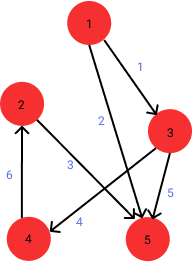
… we look for a path starting from any vertex, which visit all the vertices. The (only) path in this graph would be \(1 \rightarrow 3 \rightarrow 4 \rightarrow 2 \rightarrow 5\). The question is: How do we make use of a SAT solver to find this path?
The main idea is the following: First, we encode the problem in SAT such that satisfiable assignments to variables correspond to a Hamiltonian path. Second, we use an off-the-shelf SAT solver to solve the instance. By construction, the assignment given by the SAT solver will represent a Hamiltonian path. Third, we convert the assignments of Boolean variables to an actual path. The following figure illustrates this idea:

We start by thinking about what an assignment at the end should represent: Since we can only talk about logical relations of propositions, we should think of some propositions that would be useful considering the following:
- We want to be able to look at an assignment to all our variables, and construct a path from it trivially.
- As the path will visit vertices one by one, our propositions should somehow be related to either vertices or edges.
- A path consists of a sequence of vertices and edges. Our propositions must also relate to some ordering.
If we consider all these, one way is to use the following propositional variables $h_{ij}$ and meanings:
\[\bbox[5px, border: 2px solid black]{h_{ij}: \textrm{The } i^{th} \textrm{ vertex visited in the path is vertex } j}\]Since \(i\) and \(j\) both take values from \({1, 2, 3, 4, 5}\), we will have \(5 \times 5 = 25\) different propositions that we can talk about. At the very end, we want the SAT solver to give us an assignment to those propositions in such a way that the visited vertices constitute a Hamiltonian path. Hence, the following list contains all the propositions we will have:
\[
\begin{matrix}
h_{11} & h_{12} & h_{13} & h_{14} & h_{15} \
h_{21} & h_{22} & h_{23} & h_{24} & h_{25} \
h_{31} & h_{32} & h_{33} & h_{34} & h_{35} \
h_{41} & h_{42} & h_{43} & h_{44} & h_{45} \
h_{51} & h_{52} & h_{53} & h_{54} & h_{55} \
\end{matrix}
\]
If we give a SAT solver what we have so far, i.e., twenty five Boolean variables with an empty CNF, it is free to give us any assignment that is not constrained by anything. For instance, it can give us an assignment where both \(h_{11}\) and \(h_{12}\), which would mean that “the first vertex of the path is both vertex 1 and vertex 2”… This is nonsense, as the first vertex in a path cannot be two different vertices at the same time.
If we want to say that the first vertex of the Hamiltonian path cannot be two distinct vertices at the same time, we can use the following formula:
\[\begin{align} \label{nonsense} \tag{1} &(h_{11} \Rightarrow \neg h_{12}) \wedge (h_{11} \Rightarrow \neg h_{13}) \wedge (h_{11} \Rightarrow \neg h_{14}) \wedge (h_{11} \Rightarrow \neg h_{15}) \wedge \\ &(h_{12} \Rightarrow \neg h_{13}) \wedge (h_{12} \Rightarrow \neg h_{14}) \wedge (h_{12} \Rightarrow \neg h_{15}) \wedge \\ &(h_{13} \Rightarrow \neg h_{14}) \wedge (h_{13} \Rightarrow \neg h_{15}) \wedge \\ &(h_{14} \Rightarrow \neg h_{15}) \end{align}\]This is tedious to write, however it has a very simple structure: If we say that the first vertex of the Hamiltonian path is a certain vertex, it cannot be at the same time another vertex.
We now have a formula that expresses something that kind of describes a property of a Hamiltonian path, even though it’s missing some other properties. Just to see how this one can be fed in a SAT solver, let us discuss the input format of SAT solvers.
DIMACS format
SAT solvers read input instances from files in a format called DIMACS3. The first non-comment line of the format looks like this:
p cnf 25 10
Here we say that we have 25 variables and 10 clauses. First, we map each of our variables to a positive integer:
\[\begin{align*} &h_{11} \rightarrow 1& \\ &h_{12} \rightarrow 2& \\ &h_{13} \rightarrow 3& \\ &h_{14} \rightarrow 4& \\ &h_{15} \rightarrow 5& \\ &h_{21} \rightarrow 6& \\ &h_{22} \rightarrow 7& \\ &h_{23} \rightarrow 8& \\ &h_{24} \rightarrow 9& \\ &h_{25} \rightarrow 10& \\ &h_{31} \rightarrow 11& \\ &h_{32} \rightarrow 12& \\ &h_{33} \rightarrow 13& \\ &h_{34} \rightarrow 14& \\ &h_{35} \rightarrow 15& \\ &h_{41} \rightarrow 16& \\ &h_{42} \rightarrow 17& \\ &h_{43} \rightarrow 18& \\ &h_{44} \rightarrow 19& \\ &h_{45} \rightarrow 20& \\ &h_{51} \rightarrow 21& \\ &h_{52} \rightarrow 22& \\ &h_{53} \rightarrow 23& \\ &h_{54} \rightarrow 24& \\ &h_{55} \rightarrow 25& \end{align*}\]This mapping is arbitrary, we could have used any mapping. This is only used for encoding our variable names as integers and nothing more.
The rest of the lines encode a CNF, one clause for every line. For instance, they could be something like the following:
1 2 0
-1 -3 0
-1 -4 0
Each line here is terminated with a \(0\), and specifies a clause. In this snippet just above there are 3 clauses, with two literals each.
According to the mapping we set above, \(1\) is mapped to \(h_{11}\) and \(2\) is mapped to \(h_{12}\), hence 1 2 0 is the clause \((h_{11} \vee h_{12})\). The next line, -1 -3 0, involves negative integers mapped to negative literals, is the clause \((\neg h_{11} \vee \neg h_{13})\).
Now we can express the clauses in Formula \eqref{nonsense}:
-1 -2 0
-1 -3 0
-1 -4 0
-1 -5 0
-2 -3 0
-2 -4 0
-2 -5 0
-3 -4 0
-3 -5 0
-4 -5 0
Note that in Formula \eqref{nonsense}, we had a conjunction of implications, and we turn them into disjunctions by applying the transformation we discussed earlier to get a conjunction of clauses.
Now that we have some subset of the clauses we need, we can feed it to a SAT solver to see what it gets us.
First try
In the rest of the post I will use MiniSat, a free and open source SAT solver4. On my Debian system it was possible to install it within seconds with the command:
sudo apt-get install minisat
Then we create a file with the following contents and name it to partial1.cnf:
p cnf 5 10
-1 -2 0
-1 -3 0
-1 -4 0
-1 -5 0
-2 -3 0
-2 -4 0
-2 -5 0
-3 -4 0
-3 -5 0
-4 -5 0
Note that this file contains only a subset of the variables and the clauses we will need at the end, only enforcing that the condition that the first vertex of our path cannot be two distinct vertices at the same time. This will not get us a Hamiltonian path, but it will get us something that will be possible to fix by defining our input.
We call MiniSat as follows:
minisat partial1.cnf partial1.out
where the first argument to the executable is the input name, and the second one is the output name. This prints a bunch of statistics to the standard output, followed by a line SATISFIABLE.
If we open the file partial1.out, we have the following:
SAT
-1 -2 -3 -4 -5 0
where the first line means that a solution is found, and the second line is an encoding of the solution assignment. Each number you see is a variable, either in positive or negative form, where a positive value means that the variable is assigned to “true”, and a negative value means that the variable is assigned to “false”. Hence, this assignment corresponds to the following assignment:
\[\begin{align*} &h_{11} = \textrm{False}& \\ &h_{12} = \textrm{False}& \\ &h_{13} = \textrm{False}& \\ &h_{14} = \textrm{False}& \\ &h_{15} = \textrm{False}& \\ \end{align*}\]This is both a good and a bad result! If we remember what each of these variables meant, we see that the assignment expresses that the first vertex of our Hamiltonian path is none of the vertices we have. That means the clauses we put in the file, which were asserting that the first vertex cannot be two vertices at the same time, are satisfied. However, this did not go well as we did not end up selecting at least one vertex for this position. This is all right, as we did not let the solver know about that restriction yet. In the next few sections we will add more clauses to assert that we should select at least one vertex for each step of our path.
Note that, the clauses we added to our set only enforce that the first vertex we choose cannot be two distinct vertices at the same time (10 clauses). In our final representation, we will need to add similar clauses for all the positions (50 clauses in total). Such a listing of clauses can be examined in partial2.cnf.
Enforcing selection of at least one edge at each step
To express that we want to select at least one edge at the first step, we can write the following clauses:
\[\begin{align*} (h_{11} \vee h_{12} \vee h_{13} \vee h_{14} \vee h_{15}) \end{align*}\]which looks like this in DIMACS format:
1 2 3 4 5 0
Of course, this encforces this condition for only the first step. If we add the corresponding clause for all the steps to partial2.cnf, we get the DIMACS file partial3.cnf.
If we run MiniSat on this file, we get the following solution:
1 -2 -3 -4 -5 -6 -7 -8 -9 10 -11 -12 -13 14 -15 -16 -17 -18 -19 20 -21 -22 -23 -24 25 0
which translates to the following vertices seleced:
\[\begin{align*} &\textrm{First vertex:}& \textrm{Vertex 1} \\ &\textrm{Second vertex:}& \textrm{Vertex 5} \\ &\textrm{Third vertex:}& \textrm{Vertex 4} \\ &\textrm{Fourth vertex:}& \textrm{Vertex 5} \\ &\textrm{Fifth vertex:}& \textrm{Vertex 5} \end{align*}\]Now that we have properly selected a subset of the edges of the input graph, we can actually visualize it. The following shows the path resulting from this assignment:
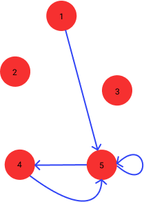
This is both good and bad again! It is good, since we have something that is a path. However, it is bad, since it’s not a Hamiltonian path (as we visit Vertex 5 three times, but never visit vertices 2 and 3 at all), or even a proper path (as the path uses edges that are not even present in the input graph).
Enforcing visiting each vertex
For this to be a Hamiltonian path, we need to visit all vertices at least once. To enforce that, we can use to following clauses:
\[(h_{1u} \vee h_{2u} \vee h_{3u} \vee h_{4u} \vee h_{5u}) \qquad \textrm{for all vertices } u\]If we add these clauses to our formulation, we get partial4.cnf. Solving again with MiniSat yields the following assignment:
` -1 -2 3 -4 -5 -6 -7 -8 -9 10 -11 12 -13 -14 -15 16 -17 -18 -19 -20 -21 -22 -23 24 -25 0 `
which translates to:
\[\begin{align*} &\textrm{First vertex:}& \textrm{Vertex 3} \\ &\textrm{Second vertex:}& \textrm{Vertex 5} \\ &\textrm{Third vertex:}& \textrm{Vertex 2} \\ &\textrm{Fourth vertex:}& \textrm{Vertex 1} \\ &\textrm{Fifth vertex:}& \textrm{Vertex 4} \end{align*}\]Let’s visualize this solution:
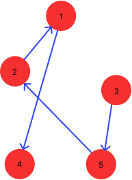
This looks much better than what we previously had! The previous visualization had the following problems:
- Some vertices that were never visited (vertex 2 and vertex 3)
- Some vertices that were visited twice (vertex 3 and vertex 4)
Adding this set of clauses were aimed at preventing problem (1), however we got lucky and prevented problem (2) as well! As we might not get always get lucky, we should add the following clauses to our formulation to enforce that no vertex is visited twice in the path:
\[\neg (h_{lu} \wedge h_{ku}) \qquad \textrm{for all } l \not= k\]which can be transformed to the following clauses:
\[(\neg h_{lu} \vee \neg h_{ku}) \qquad \textrm{for all } l \not= k\]After adding these to our formulation, we get partial5.cnf. Solving with MiniSat gets us:
1 -2 -3 -4 -5 -6 -7 8 -9 -10 -11 -12 -13 14 -15 -16 17 -18 -19 -20 -21 -22 -23 -24 25 0
which translates to:
\[\begin{align*} &\textrm{First vertex:}& \textrm{Vertex 1} \\ &\textrm{Second vertex:}& \textrm{Vertex 3} \\ &\textrm{Third vertex:}& \textrm{Vertex 4} \\ &\textrm{Fourth vertex:}& \textrm{Vertex 2} \\ &\textrm{Fifth vertex:}& \textrm{Vertex 5} \end{align*}\]and which looks like the following when we visualize it:

This actually is a Hamiltonian path! However, this is a bit fishy… If you go back and review all the clauses we added to our formulation, you will see that none of our clauses drew information from the edges of the input graph, and there is no way for the solver to know about the edges we have in our input graph. Still, it got the right answer somehow.
Something similar to what happened in the previous step just happened: The solver just got lucky, and gave us a solution that really was a Hamiltonian path. If we were not this lucky, or ask for not just one solution but a second one, the solver would give us a solution that follows inexistent edges.
To show that there are other solutions than the one we just got, we will temporarily enhance our formula with a clause excluding the first solution. This is just a trick to see another solution the solver might have found, and we will remove this clause later on.
Here is the formula that describes the solution we got:
\begin{aligned}
(\phantom{\neg }h_{11} \wedge& \neg h_{12} \wedge \neg h_{13} \wedge \neg h_{14} \wedge \neg h_{15} \ \wedge \
\neg h_{21} \wedge& \neg h_{22} \wedge \phantom{\neg} h_{23} \wedge \neg h_{24} \wedge \neg h_{25} \ \wedge \
\neg h_{31} \wedge& \neg h_{32} \wedge \neg h_{33} \wedge \phantom{\neg} h_{34} \wedge \neg h_{35} \ \wedge \
\neg h_{41} \wedge& \phantom{\neg} h_{42} \wedge \neg h_{43} \wedge \neg h_{44} \wedge \neg h_{45} \ \wedge \
\neg h_{51} \wedge& \neg h_{52} \wedge \neg h_{53} \wedge \neg h_{54} \wedge \phantom{\neg} h_{55}\phantom{\wedge} \ )
\end{aligned}
Since we want to discard this particular assignment, we negate it:
\begin{aligned}
(\neg h_{11} \vee \ & \phantom{\neg} h_{12} \vee \phantom{\neg} h_{13} \vee \phantom{\neg} h_{14} \vee \phantom{\neg} h_{15} \ \vee \
\phantom{\neg} h_{21} \vee \ & \phantom{\neg} h_{22} \vee \neg h_{23} \vee \phantom{\neg} h_{24} \vee \phantom{\neg} h_{25} \ \vee \
\phantom{\neg} h_{31} \vee \ & \phantom{\neg} h_{32} \vee \phantom{\neg} h_{33} \vee \neg h_{34} \vee \phantom{\neg} h_{35} \ \vee \
\phantom{\neg} h_{41} \vee \ & \neg h_{42} \vee \phantom{\neg} h_{43} \vee \phantom{\neg} h_{44} \vee \phantom{\neg} h_{45} \ \vee \
\phantom{\neg} h_{51} \vee \ & \phantom{\neg} h_{52} \vee \phantom{\neg} h_{53} \vee \phantom{\neg} h_{54} \vee \neg h_{55}\phantom{\vee} \ )
\end{aligned}
If we add this to partial5.cnf, and solve it, there are two possibilities:
- The solver reports that the instance is unsatisfiable, meaning that the
solution we got for the original
partial5.cnfwas the only one. - The solver reports a solution, meaning that it is another solution of
partial5.cnf
Here is what we get from MiniSat:
` -1 -2 -3 4 -5 6 -7 -8 -9 -10 -11 -12 -13 -14 15 -16 -17 18 -19 -20 -21 22 -23 -24 -25 0 `
This is what we see when we visualize it:
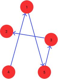
So, this is another solution of partial5.cnf, however it is completely bogus!
Even though it is a path that visits all the vertices in the input graph, the edges
in the path do not actually exist. In the next section, we will let our
formulation to use only edges that are in the input graph.
Enforcing that the path consists of real edges
For our satisfying assignments to represent real paths, for each successive pair of vertices, we need the following constraints to hold for all \(i \in \{1,2,3,4\}\):
\[\neg (h_{iu} \wedge h_{(i+1)v}) \qquad \textrm{ if there is not an edge between } u \textrm{ and } v\]If we push the negation through, we get the following formulas:
\[(\neg h_{ui} \vee \neg h_{(i+1)v}) \qquad \textrm{ if there is not an edge between } u \textrm{ and } v\]which are clauses, and we can add them to our formulation to get hamiltonian.cnf. If we solve this with MiniSat, we get the following assignment:
` 1 -2 -3 -4 -5 -6 -7 8 -9 -10 -11 -12 -13 14 -15 -16 17 -18 -19 -20 -21 -22 -23 -24 25 0 `
corresponding to the following path:
\[\begin{align*} &\textrm{First vertex:}& \textrm{Vertex 1} \\ &\textrm{Second vertex:}& \textrm{Vertex 3} \\ &\textrm{Third vertex:}& \textrm{Vertex 4} \\ &\textrm{Fourth vertex:}& \textrm{Vertex 2} \\ &\textrm{Fifth vertex:}& \textrm{Vertex 5} \end{align*}\]This is the same solution we got for partial5.cnf! However, this time if we
add the negation of this assignment to the formulation we will see that there
are no solutions exist, which matches our expectation.
This completes our formulation of the Hamiltonian path instance in SAT.
Conclusions
In this post we explored how we can formulate a combinatorial problem, the Hamiltonian path problem, in the language of Boolean Satisfiability.
This is a tedious, yet easy process:
- Start with some logical formula that discards some structure that you do not want to see in the solution.
- Solve the partial formulation with a solver, examine the output and identify properties that you would not like to see.
- Repeat until you get a SAT solution that represents a valid solution to your original problem.
For non-trivial instances, one almost always writes a script to generate the CNF
file from your input data, otherwise keeping track of your variables becomes very
difficult. You can see a sample script to generate hamiltonian.cnf here.
One of the interesting things about this paradigm is that when you get a solution that is wrong, debugging is a completely different procedure than how you would debug a program you implement with a general purpose programming language. In this paradigm, you only add or remove constraints in a declarative way. This does not mean that debugging SAT instances are always easier than debugging a traditional program, however I would very much prefer writing out a SAT formulation than writing a C++ program that does the same thing.
The formulation I present here, of course, is not the only way to encode the Hamiltonian Path Problem in SAT. There could be many other formulations, including more efficient ones. However, the one I present here is probably one of the easiest ones to understand.
One important question regarding this paradigm is the following: If we can encode any problem in NP as a CNF, how can we encode non-binary values as propositions? For instance, in the Traveling Salesman Problem (TSP) one has to consider distances between cities, and it is not clear how one can easily encode integer distances in SAT. I will leave the answer for another post!
If you have any comments, or questions, do not hesitate to contact me on Twitter.
Notes
-
More interestingly, we can also say \((F \equiv G) \equiv ((F \Rightarrow G) \wedge (G \Rightarrow F))\) is true for all formulas under all assignments. ↩
-
There is an encoding called Tseitin’s transformation that is guaranteed to produce only a polynomially longer CNF. ↩