Formulating the Hamiltonian Path Problem as a Constraint Satisfaction Problem
My previous blog post demonstrates how we can formulate the Hamiltonian Path Problem as an instance of the Boolean Satisfiability Problem (SAT). Once you have the formulation, it is very easy to use a solver (such as MiniSat) to solve it.
However, for most problems it is a tedious job to manually write the SAT encoding. For this reason, it is common to write scripts in a programming language that generate them automatically.
One other option for solving such an NP-complete problem is expressing it as a Constraint Satisfaction Problem (CSP). You can think of CSP as a generalization of SAT with two distinct features:
- In a CSP you have not only binary propositions, but also variables over arbitrary finite domains
- A CSP also considers more powerful constraints, such as arithmetic constraints, linear equalities/inequalities, cardinality constraints, etc.
That is, the input languages to the CSP solvers are much more expressive, as they let us talk about many other things than propositions and Boolean clauses.
You might expect that as we increase the expressivity of our constraint language, the computational complexity of finding a solution would increase as well. However, for many useful constraints (including the ones that we will mention in this blog post) the complexity is still NP-complete1.
In this post, we will explore how we express the Hamiltonian Path Problem as a CSP instance, and solve it using a CSP solver. By doing so, we will demonstrate that it is possible to get a much expressive (and shorter) formulation of the Hamiltonian Path Problem than our previous SAT encoding.
MiniZinc language
MiniZinc language is a constraint modeling language that can be used to express CSPs. Similar to what we have done for SAT in my previous blog post, we can use an off-the-shelf solver to solve the CSP to get a solution to the Hamiltonian Path Problem.
Here is what a variable declaration looks like in MiniZinc:
var int: x;
which declares an integer2 variable called x.
You can model a finite domain variable with the following:
var 0..2: y;
which declares a variable y that can take values from the set \(\{0, 1, 2\}\).
You can also declare arrays of variables with the following syntax:
array [1..4] of var 1..5: xs;
which declares a variable array of size 4 called xs, each taking values from the set \(\{1, 2, 3, 4, 5\}\).
You can omit the keyword var in the above examples to declare constants:
int: constant_x = 3;
array[1..4] of 1..5: constant_xs = [5, 4, 3, 2];
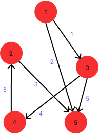
Now that we can talk about variables, let us think of what variables we will need to find a Hamiltonian path in the following graph:
Recap of the SAT formulation
In our SAT formulation here, we had the following binary variables:
\[\bbox[5px, border: 2px solid black]{h_{ij}: \textrm{The } i^{th} \textrm{ vertex visited in the path is vertex } j}\]and we had the following classes of constraints:
- Each step of the path is mapped to at most one vertex
- Each step of the path is mapped to at least one vertex
- Each vertex is visited at least once
- The path can visit a vertex only if there is an edge to it from the previous vertex
In the rest of the post, I will refer to these classes as (C1), (C2), (C3), and (C4).
CSP Variables
Since CSP is a generalization of SAT, we can still use the same variables to formulate a CSP. However, we can come up with a much more succinct representation as we can use arbitrary finite domain variables in a CSP.
In our SAT formulation, \(h_{ij}\) being true meant that the \(i^{th}\) vertex in our output path is vertex \(j\). What we were trying to do was actually mapping each order index to some vertex. When you think about variables and assignments, an assignment is also a mapping to a set of variables. This hints that what the SAT encoding was doing was actually imitating assignments to a variables that we never had in the first place! If we represented each order in the path as a variable with a domain of \(\{1, 2, 3, 4, 5\}\), that would all be what we need. That is:
array[1..5] of var 1..5: path;
We have an array of 5 variables, as our path should be of size 5. The domain of each of these variables is 1..5 as we have 5 vertices to choose from.
Solving with a CSP solver
MiniZinc is not only a language, it is also a compiler that compiles the MiniZinc language to a simpler form called FlatZinc. Many CSP solvers recognize the FlatZinc format, so we will need to utilize the compiler to solve our CSP.
The MiniZinc compiler is bundled with 3 different solvers:
- Gecode, a traditional CSP solver
- Chuffed, a clause learning CSP solver
- Cbc, an integer programming solver
To solve such a simple Hamiltonian Path Problem instance, any of these solvers will suffice. In this post I will be using Gecode.
Once you have MiniZinc installed3, let us use it to solve the following file that only contains our variable declaration:
array[1..5] of var 1..5: path;

solve satisfy;
In the second line, we tell the solver to solve it only to satisfy it, in constrast to optimizing the value of a variable.
After saving the above statements to a file called partial1.mzn, we call Gecode with the following commandline:
minizinc --solver gecode partial1.mzn
to get the following:
path = array1d(1..5, [1, 1, 1, 1, 1]);
The most important part of the output is [1, 1, 1, 1, 1], which is the path array we were looking for. To format things a bit, we can add the following to the end of the file:
output ["Path: " ++ show(path)];
to get a more readable output:
Path: [1, 1, 1, 1, 1]
Note that just one line of declaration captures the constraints of classes (C1) and (C2) without any hassle. One obvious problem is that this omits the constraints of class (C3), leading to a path that only consists of vertex 1. In the next section we will fix that.
Visiting each vertex
In a CSP, we can express the following 5 clauses for the constraints of class (C3):
\[(path[1]=1) \vee (path[2]=1) \vee (path[3]=1) \vee (path[4]=1) \vee (path[5]=1) \\ (path[1]=2) \vee (path[2]=2) \vee (path[3]=2) \vee (path[4]=2) \vee (path[5]=2) \\ (path[1]=3) \vee (path[2]=3) \vee (path[3]=3) \vee (path[4]=3) \vee (path[5]=3) \\ (path[1]=4) \vee (path[2]=4) \vee (path[3]=4) \vee (path[4]=4) \vee (path[5]=4) \\ (path[1]=5) \vee (path[2]=5) \vee (path[3]=5) \vee (path[4]=5) \vee (path[5]=5)\]which are the very same constraints that we had in the SAT formulation, only with integer variables rather than propositional variables.
However, CSPs let us express what we actually want with only a single constraint, called the “alldifferent constraint”. The semantics of the constraint is what you would expect: If we say that a set of variables are “alldifferent”, they must take different values in the solution. In MiniZinc, we write it as:
constraint alldifferent(path);
Since this is a part of the MiniZinc standard library, we add the following line to include it:
include "alldifferent.mzn";
After we add these two lines to partial1.mzn, we get partial2.mzn. Solving it with Gecode shows:
Path: [5, 4, 3, 2, 1]
This is effectively a permuation of our input nodes! If you want to see all solutions to this formulation, you can see them with:
minizinc --solver gecode --all_solutions partial2.mzn
Note that the constraints of class (C3) are not the same thing as the alldifferent constraint, however after they are combined with (C1) and (C2), an alldifferent constraint over the path variable amount to the same thing. Now that we have a proper permutation of our input vertices, the only remaining thing to express is to only visit a new vertex only if there is an edge to it from the previous vertex.
Predicates and abstractions
Since we are interested in finding a path in a specific graph, we should somehow include it to the formulation. One way of doing that in MiniZinc is to declare them as constants:
array[1..6] of 1..5: source = [1, 1, 2, 3, 3, 4];
array[1..6] of 1..5: target = [3, 5, 5, 4, 5, 2];
Note that we omitted the keyword var in these declarations to declare source and target as constants.
What we want to express next is the following logical statement for all \(u, v\):
\[(\textrm{There is not an edge between } u \textrm{ and } v) \Rightarrow (u \textrm{ cannot precede } v)\]To formalize it a bit, we would need two “predicates” that capture the meanings above:
\[\neg edge(u, v) \Rightarrow \neg precedes(u, v)\]Let us think about the predicate \(edge(u, v)\) in mathematical terms, and we will see how we can translate that to MiniZinc. Given the constant arrays source and target, what we want is the following:
where $E$ is the set of our input graph’s edges, which could be represented as the index set \(\{1,2,3,4,5,6\}\).
If you are convinced that this is a nice definition of the \(edge(u,v)\) predicate, here’s how MiniZinc lets us express the same thing:
predicate edge(int: u, int: v) =
    exists(e in 1..6)(source[e] == u /\ target[e] == v);
which is almost at a one-to-one correspondence with the mathematical notation. After this declaration, we can use this predicate wherever we need.
The other predicate we want, \(precedes(u,v)\), can be defined as follows mathematically:
\[precedes(u, v) = \exists i \in [1,4]\ldotp(path[i]=u \wedge path[i+1]=v)\]Similarly, MiniZinc lets us do this definition with the following syntax:
predicate precedes(int: u, int: v) =
    exists(i in 1..4)(path[i] == u /\ path[i + 1] == v);
Now that we have the definitions for our ingredients of our constraints expressing (C4), we can use the following implication constraint:
constraint forall(v1, v2 in 1..5)(not edge(v1, v2) -> not precedes(v1, v2));
If we add these three lines to the previous forulation, we get hamiltonian.mzn. Solving it yields:
Path: [1, 3, 4, 2, 5]
which is a Hamiltonian path in our input graph! With the all-solutions commandline flag, you can also verify that this is the only path that can be found in the graph.
Conclusion
In this post, we explored how we can solving a Hamiltonian Path Problem instance by formulating it as a CSP. Compared to the SAT formulation, this is much more expressive, much easier to understand, and much easier to modify.
Note that, the formulation that I present in this blog post is not necessarily the only or the most efficient way to solve it in MiniZinc language. MiniZinc is an extensive language, and mastering it takes a lot of time and practice. If you want to read more about MiniZinc, here are two very good official resources:
Also, the problem instance we solve here is very tiny, compared to what you can solve with a good CSP solver. In practice, such solvers can handle millions of variables and constraints.
Do all these mean that CSP is always a better option than SAT? Absolutely not, as these two formalisms have their own advantages. SAT solvers are still very good options for solving certain problems, and many such solvers utilize a lot of sophisticated techniques that do not necessarily exist in a CSP solver.
Hope you enjoyed this post! As always, feel free to reach me on Twitter for any questions or comments.
Notes
-
For instance, if checking the satisfaction of one of your supported constraints is not in P, then your CSP will surely not be an NP-complete problem. ↩
-
In practice, solvers model integer variables as finite domain variables with a very large domain. Also, it is usually possible for us to derive lower and upper bounds for all variables ourselves. ↩
-
You can install Minizinc from here. Debian and Ubuntu package repositories seem to have
minizincpackages, however they seem to be outdated a bit. ↩